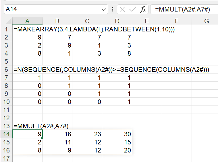
To calculate a 2-D array where each row is the cusum of each row in the source table, it’s possible to use the MMULT function. The matrix multiplication is done with an upper-right triangular array of 1s. That’s fine for a small number of columns, like 12. Using a lower-left matrix, you can calculate cusums down the columns. But when you get to 1000 rows, the matrix is a million-cell array, and for 3000 rows or more, Excel is going to go out of memory. I asked on LinkedIn for suggestions for an efficient method of doing this for a dynamic array cusum down columns.
We have a winner.
I have a dynamic array of 4000 rows and 4 columns in A3.
A3# is =MAKEARRAY($K$1,4,LAMBDA(I,j,I*10+j))
K1 contains 4000 – a number which causes the MMULT formula to run out of resources, its max was 3000.
I put 100 recalculations of each cusum formula below in a loop, and timed it with Charles Williams’s Microtimer function.
The winner is Diarmuid Early’s 2nd suggestion in the LinkedIn thread but in column order
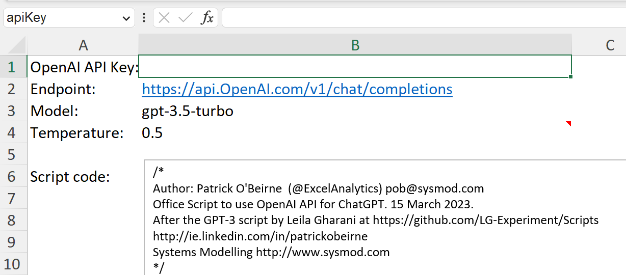
Everybody seems to want to use AI to create Excel formulas, so here is a way of building an interface to the OpenAI ChatGPT 3.5 model. Leila Gharani has already published a video and the Office Script code to call the GPT-3 API. This is for ChatGPT 3.5 which has a different data structure in the JSON.
I did this as an exercise in learning Excel scripting, which is based on Typescript, with some limitations both on the language features and the amount of access it has to the Excel Object Model.
You can download the ChatGPT in Excel demo workbook here. It has two sheets, The API sheet is where you fill in the API key you get when you sign up on openai.com, and it contains the script as plain text. The ChatGPT sheet is where you put in the prompts and then run the script to get the answer.
When working on VBA code that should work in both MSExcel and MSAccess VBA, the different application object methods can be hard to manage. For example, Application.Screenupdating = False is used in Excel but would raise a compile error in Access. The workaround is to use late binding so the host application will not check the validity of the methods until runtime. In the code below, I would use SetScreenUpdating(False) instead, and that code will work in both Excel and Acess.
Option Explicit
' Functions to apply system commands in either host using late binding for Application object
Private Const MSACCESS As String = "Microsoft Access"
Private Const MSEXCEL As String = "Microsoft Excel"
Function SetScreenUpdating(bOnOff) As Boolean
Dim oApp As Object: Set oApp = Application
Static bSetOnOff As Boolean
If oApp.Name = MSACCESS Then
' no way to get the status, just return the last status set
SetScreenUpdating = bSetOnOff
bSetOnOff = bOnOff
oApp.Echo bOnOff
ElseIf oApp.Name = MSEXCEL Then
SetScreenUpdating = oApp.Screenupdating
oApp.Screenupdating = bOnOff
End If
End Function
Function SetHourGlass(bOnOff) As Boolean
Dim oApp As Object: Set oApp = Application
If oApp.Name = MSACCESS Then
SetHourGlass = oApp.Screen.MousePointer = 11 ' 11 Busy (Hourglass) 1=Normal 0=Default
oApp.DoCmd.Hourglass bOnOff
ElseIf oApp.Name = MSEXCEL Then
SetHourGlass = oApp.cursor = 2
oApp.cursor = IIf(bOnOff, 2, -4143) ' xlwait=2, xldefault=-4143
End If
End Function
Sub testApp()
SetHourGlass True
SetScreenUpdating False
MsgBox "hi"
SetScreenUpdating True
SetHourGlass False
End Sub
Victor Momoh in the Global Excel Summit, to start a discussion on readability, provocatively used MMULT in a formula to determine whether a word contains all five vowels. As Victor said, in real life he’d use a simple SUM: =SUM(1*ISNUMBER(SEARCH(MID(“aeiou”,SEQUENCE(1,5),1),A2)))
SEQUENCE generates {1,2,3,4,5}. The MID returns an array of each letter in “aeiou”. As Rick Rothstein pointed out, the formula would be even simpler with that array written out literally:
The SEARCH checks where the letter occurs in the word in A2 and returns a number if present or #VALUE! if not. ISNUMBER converts that to a True or False. 1* converts them to 1/0. SUM adds the array up so if it’s 5, then all five vowels are present (eg in “sequoia”).
To use this as a filter for a list of words in A2:A30000 : =FILTER(A2:A300000,BYROW(A2:A300000,LAMBDA(word,5=SUM(1*ISNUMBER(SEARCH(MID(“aeiou”,SEQUENCE(1,5),1),word))))))
The FILTER function outputs a dynamic array of the rows in a given range that match a condition.
If column B contains numbers, to get a list of the values in column A where B is greater than 3, use =FILTER(A2:A100,B2:B100>3). Because this is a dynamic array function, you only need to enter it once and its output expands to the number of matching values.
To filter for words containing one letter, we can use =FILTER(A2:A30000,ISNUMBER(SEARCH(“a”,A2:A30000)))
However we can not use an array eg {“a”,”e”} for the SEARCH first argument as that would generate a two dimensional array which would not fit the one dimension that the filter requires. You can verify that by entering =SEARCH({“a”,”e”},A2:A30000) in a cell. We want to restrict the scope of the search to each word, each row of the words list. To do that we use the BYROW function.
A LAMBDA is a user defined function in Excel, it does not involve VBA. The function we use takes one argument, given the arbitrary name “word” and that word is searched for each vowel in turn and the sum of the successful searches is calculated.
To make this easier to read, I’ll modify the formula above, which uses LAMBDA directly (that’s called an ‘anonymous’ function) to use a named function UniqueVowelCount() which we define ourselves by creating a Name as follows:
=UniqueVowelCount(“Excel”) returns 1, there is one distinct vowel “e” in the word, twice.
So now we can use BYROW to pass each row of A2:A30000 to the UniqueVowelCount function to create a one-column array of vowel counts and pass the result of comparing each with 5 to the FILTER function
which you can evaluate using the Formula Auditing tab, Evaluate Function button.
P.S. Not that anyone asked, but in the SOWPODS corpus (now called the Collins Scrabble (TM) word list) there are 2,932 words of less than 15 letters with all five vowels.
I didn’t like the idea of using recursion where simple looping through the string would do, so I wrote this Slugify(text) user-defined function using a LAMBDA. It converts the text to lowercase and then to an array, iterates through all the characters in the array passing them to another LAMBDA function AlphaNum(char) to return a space if the character is not a-z or 0-9, and finally concatenates the array back to a string.
Because AND() and OR() return single values and cannot be used in an array function. So I use Boolean * for AND and + for OR.
Bill Jelen showed a neat trick to reduce multiple occurrences of a character: change all occurrences of that character to a space, then use TRIM to reduce all spaces to one, then substitute back. Here I use spaces to begin with, then substitute them with a dash at the end.
Of course, the only use for LAMBDA is to create a nice encapsulated user-defined function. If you want a non-LAMBDA formula on a direct cell reference eg A3, just use a simple LET:
Why does this work: =LET(A,A1:A10,B,A+1,COUNTIFS(A,”<5″)); it returns a count.
But this does not: =LET(A,A1:A10,B,A+1,COUNTIFS(B,”<5″)); it returns #VALUE!.
The reason is that all the IFS functions only accept a range as their first parameter, not an array. So for example =COUNTIFS({1,2,3,4,5,6},”<5”) gives a syntax error, an invalid formula.
The solution is to use FILTER() to select the values you want, then use COUNT or AVERAGE or whatever you want on that.
You know that feeling when a manufacturer pulls the rug from under you? When a feature (OK, a workaround, even a hack) you’ve been relying on for years suddenly stops working because of an “upgrade”? Welcome to the world of the VBA developer in an Apple environment.
Excel VBA macros can be launched by keystroke shortcuts such as Ctrl+q, Ctrl+Shift+q, Ctrl+Alt+q. For example, Application.OnKey “^%q”, “MyMacro” is launched by Ctrl+Alt+q.
That works fine in Windows. But Excel for Apple Mac VBA does not detect the Command or Option (same as Alt) keys. There used to be a workaround, posted by Ron de Bruin on macexcel.com which used the Cocoa library in Python to return the modifier keys pressed. My version is
BUT in the latest MacOS upgrade, Monterey, Python is no longer built in. Apple has officially deprecated Python 2.7 in macOS Monterey 12.3. “The company is advising its developers to use an alternative programming language instead, such as Python 3, which, however, does not come preinstalled on macOS.”
I posted a question “Is there a newer/better way to detect what modifier keys are being pressed?” at https://macscripter.net/viewtopic.php?pid=209786 and got a very helpful reply from Nigel Garvey.
Here’s the MacScript version. Multiple lines are separated by both return & linefeed characters.
scpt = "use framework ""AppKit""" & vbCrLf
scpt = scpt & "return current application's class ""NSEvent""'s modifierFlags()"
Debug.Print MacScript(scpt)
However, in the future we may have to use the more awkward AppleScript function. The MacScript function has been deprecated, therefore it is no longer supported (although at the time of writing it is still present in Office for Mac VBA). For more information, see this Stack Overflow article.
The script needs to be put in a .scpt file in a hidden folder in the user’s home folder: /Users/username/Library/Application Scripts/com.microsoft.Excel. The file looks like the following; from testing I found that of the “use” statements, only the AppKit line is essential.
use AppleScript version "2.4" -- Yosemite (10.10) or later
use framework "Foundation"
use framework "AppKit"
use scripting additions

on modifierKeysPressed()
   return current application's class "NSEvent"'s modifierFlags()
end modifierKeysPressed
It is invoked by the AppleScriptTask function, eg AppleScriptTask("modifierKeysPressed.scpt", "modifierKeysPressed", ""). This is unfortunately quite slow, from 0.7 seconds to several seconds, I found when testing.
If you play Wordle daily, or the French version LeMot, you might want to practice more often. For fun, I created an Excel version that you can download, WordXLe, and a Wordle Solver. It has sheets for both English and French versions. It requires an Excel 365 subscription because it uses the dynamic array functions. If you don’t have Excel 365, you can still use the Google sheets version of the Wordle Helper. Be sure to Save a Copy so you can edit the copy.
The workbooks were last updated 27 April, 2022. Be sure you have the latest version! UPDATE 9 Feb 2022: BYROW function and LAMBDA make the formulas more manageable.
UPDATE 3 May 2022: Wordle Helper 4.0 released. (Downloads: http website, insecure or Dropbox download, secure.) This requires the latest Excel 365 version because it uses the BYROW and LAMBDA functions. It uses the same grid layout as Wordle so should be more familiar. You set the colour of a cell by clicking its spinner. The colour scheme is configurable. Let me know if you find it better!
It uses Conditional Formatting for colouring, Data Validation to enforce some letter entry rules, no VBA macros, just formulas. The sheets are protected, but it’s easy to unhide things in Excel if you really want to so I’ll leave that as a challenge.
CAUTION: Always ensure that this is the first workbook you open after starting Excel, and that you close without saving and exit Excel when finished the game. This workbook uses iteration to randomly select a hidden word. If any other workbook is open before this is opened, that will probably prevent this from working. If Excel gives a warning about circular references when you complete the first word, click File > Options > Formulas and check “Enable iterative calculation”. When finished, close this workbook without saving it, and close Excel, to avoid the iterative calculation setting of this workbook affecting any subsequent ones you open.
How to play: Enter one letter per cell, one valid 5-letter word per row. This version recognises about 12000 words but only 1100 are in the selection for playing. The cells change colour, following the Wordle scheme for colour-blind vision: Orange: correct letter in the correct place. Blue: a letter in the word but not in the correct place. Grey: incorrect letter. Do not change a word once entered. Work down the rows until you get them all correct. If you want some help, click the “Show Hints” checkbox to see a list of words (max 100) that fit your letters so far. If you cannot do it on the sixth row, the answer will appear in the right hand column.
Wordle Helper
By popular demand I give a Wordle helper workbook for Excel 365 with sheets for both English and French. Right-click the link and download it. Or, use my Google Sheets Wordle Helper; save a copy so you can edit your own copy.
On the language sheet you want, enter the letters you know so far and it will show you the words that fit that selection. Handy for when you have only one guess left! Here is how it works:
Think of this as a text searching problem that could be used in other scenarios. You might have part codes or account codes where there may have been transcription errors and you want to find out what the entry should have been.
We start with a list of known words. Wordle has a list of 12970 words. I use a list of12478. In the game, we know three things about the letters in each of your guess words: 1) Those in the correct place in the unknown word; they are on green tiles. 2) Those present in the unknown word but not in the correct place; they are on yellow. 3) Those not in the unknown word; they are on grey.
So the Helper has to match the words in the complete word list with the letters know to be in or not in the word. In Excel 365, we have the FILTER() function which dynamically filters a list. It is not in Excel 2019, 2016 or older. https://support.microsoft.com/en-us/office/filter-function-f4f7cb66-82eb-4767-8f7c-4877ad80c759 =FILTER(range, criteria, ifempty) The range is our list of words, for example in W1:W12478. The criteria expression tests each word and returns a True to include it in the filtered list, False to exclude it. So we could show all words beginning with “A” like this: =FILTER(W1:W12478, LEFT(W1:W12478,1)="A","") The final “” parameter is for the function to return an empty string rather than #CALC!
From now on, I’ll use the range name “en” to refer to our English dictionary list.
Let’s set up five cells and place the known correct letters in each of the five cells. Suppose we have five cells A2:E2 as shown in the picture above. Our test for the exact correct first letters then is =FILTER(en,LEFT(en,1)=A2,””)
Now to test two letters. We want the filter to include only words where both letters are in the right place. You might think we could use AND( LEFT(A1,1)=A2 , MID(en,2,1)= B2) But unfortunately AND does not work with arrays. =AND({TRUE,TRUE},{TRUE,FALSE}) returns only one result, FALSE, not the expected {TRUE, FALSE} The way to combine them with AND is to multiply the two tests. Multiplication returns a numeric result where 1=True, 0=False. ={TRUE,TRUE}*{TRUE,FALSE} returns {1,0} So our formula now is (I’ve changed the LEFT to MID for consistency) =FILTER(en, (MID(en,1,1)=A2) * (MID(en,2,1)=B2) ,””)
However, if either A2 or B2 is blank, that will fail, as a letter does not match a blank. So we extend the test by allowing any cell to be empty.
The SEARCH function does a case-insensitive search of one string inside another. =SEARCH(“a”,”start”) returns 3 If you search for an empty string, it always returns 1. =SEARCH(“”,”start”) returns 1 If you search for a string NOT in the searched string, it returns an error value. =SEARCH(“x”,”start”) returns #VALUE! Therefore to get a simple True/False, we use ISNUMBER() around the search so any numeric result of the search is True and any error is False. We multiply all the search results together as they must all be true for this first set. We only need one ISNUMBER because search with an empty cell always returns 1. To make such a long formula easier to read, press Alt+Enter after each subexpression so it finally reads
Secondly we want to filter words containing letters that we know are in the target word, although not necessarily in the position of our guess. We put all these letters into one cell, G2. There cannot be more than five of these letters. The following formula returns all the words containing the first letter of G2.
=FILTER(en,ISNUMBER(SEARCH(MID(G2,1,1),en)))
We want to apply this filter to the output of the previous filter. Rather than make the first formula even longer, we’ll create a new formula and its input range is the output of the first filter. If the first filter is in I3, then its spilled dynamic range is referred to as I3#.
=FILTER(I3#,ISNUMBER(SEARCH(MID(G2,1,1),I3#)))
Now to extend the formula to cover up to five letters in G2. We put this in J3:
=FILTER(I3#,ISNUMBER(
 SEARCH(MID(G2,1,1),I3#)
*SEARCH(MID(G2,2,1),I3#)
*SEARCH(MID(G2,3,1),I3#)
*SEARCH(MID(G2,4,1),I3#)
*SEARCH(MID(G2,5,1),I3#)),"")

With BYROW() based on J3# above :
=FILTER(I3#,BYROW(ISNUMBER(
 SEARCH(MID(G2, SEQUENCE(1,5),1),I3#)),
 LAMBDA(array,PRODUCT(--array))))
Finally we consider the letters which are NOT in the hidden word. There could be at most 21 of these, but let’s take a sensible limit at 15. We can put them all into one cell, say H2. We want to exclude any word containing any of these letters. In other words, we include any word where the search for the letter returns an error. we use ISERROR instead of ISNUMBER.
A complication is that ISERROR(SEARCH(MID(H2,1,1),J3#)) will return False if H2 is empty, because SEARCH will return 1. So we ensure the test string is padded to at least fifteen characters as follows: In K2, put =H2&REPT(“@”,15) and now use K2. Put this in L2, using the filter result from J3.
=FILTER(J3#,
 ISERROR(SEARCH(MID(K2,1,1),J3#))
*ISERROR(SEARCH(MID(K2,2,1),J3#))
... *ISERROR(SEARCH(MID(K2,15,1),J3#)),"")

Version with BYROW() :
=FILTER(J3#, BYROW(
 ISERROR(SEARCH(MID(K2, SEQUENCE(1,15),1),J3#)),
 LAMBDA(array,PRODUCT(--array))
))
Now we have the complete filter result.
See the workbook “WordleHelper.xlsx“. The intermediate columns I:K are hidden for tidiness but the sheets are unprotected. The BYROW version is not uploaded yet, until BYROW is generally available to all Excel 365 users. You have the formulas above.
Today we rolled out lambda function support to Excel users on the current channel. If you use dynamic arrays, I’d recommend starting with BYROW and BYCOL which can be used to aggregate rows/columns and spill the results. Announcing LAMBDAs to Production and Advanced Formula Environment, A Microsoft Garage Project
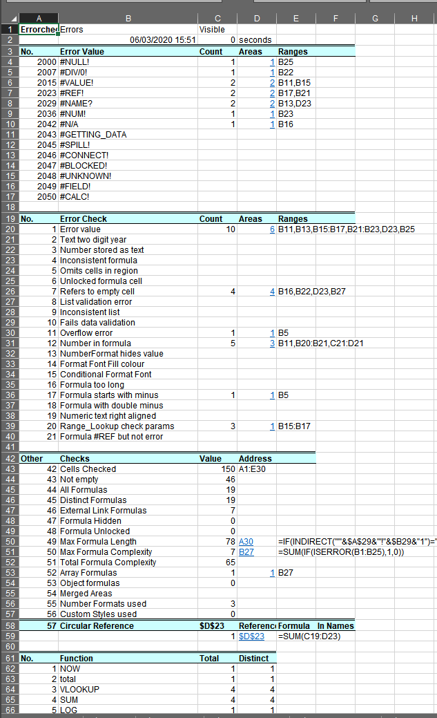
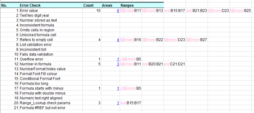
I have released an update to my XLTest Excel add-in for spreadsheet auditing, visualisation, and testing.
Changes up to version 1.74 (September 2021)
Start Session dialog changed to show internal workbook information before opening, and to open in manual calculation to prevent recalculation.
Start can remove sheet protection from unprotected OpenXML files to simplify processing.
Reports legacy BIFF properties in xls files to sheet $FileDoc.
Handles Unicode file and folder names.
Warns on unusual range name reference starting with “=!”.
New #Error values (#SPILL! etc) are reported in the detailed inspection.
Right-click shortcut to filter where-used listings for Names, Styles, Links.
Performance improvements.
VBA performance timing at procedure and optionally line level.
Detailed documentation reveals all the non-obvious content of the spreadsheet. It can reveal hidden rows, columns, and sheets. It helps you get to grips with a large spreadsheet that you have to understand.
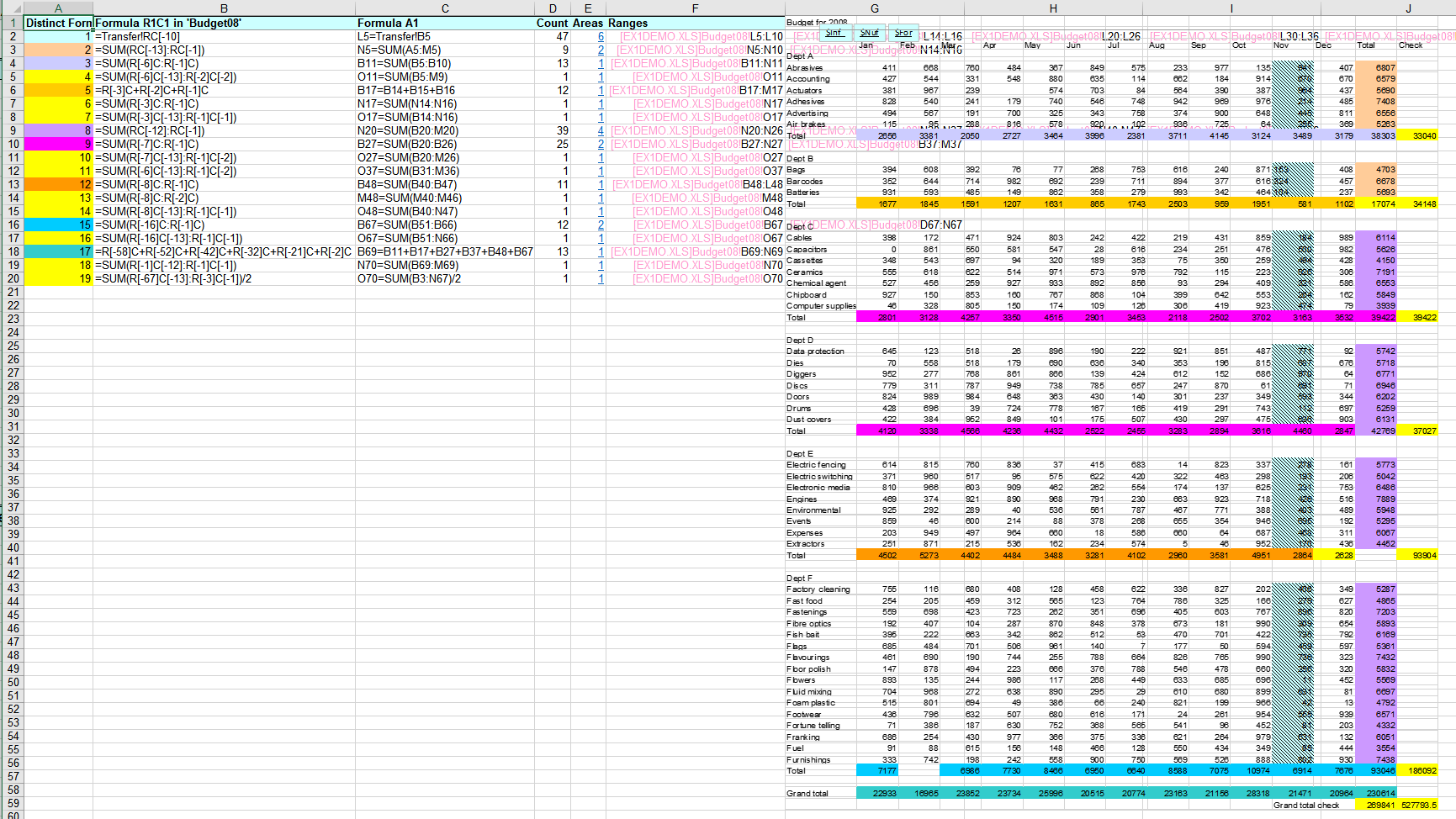
Colour maps give you an easily readable visualization of the structure and content of a spreadsheet. Inconsistent formulas and data stand out for attention.
Detailed error checking makes it easy to find and fix errors far more quickly than with tedious cell-by-cell inspection.
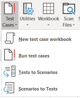
Test case maintenance and documentation make it easy to prove regression testing
Utilities provide more ways to test, such as profiling VBA performance.
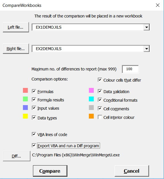
Worksheet and workbook comparisons make it easy to see what has changed between two versions of a spreadsheet file
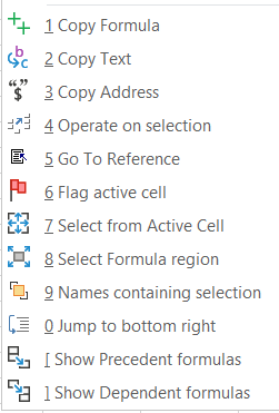
Convenient keyboard and menu shortcuts make navigation and operations easier
Quickly scan folders of Excel files to create an inventory of spreadsheets and their statistics to assist in risk assessment
For a complete manual, pricing, and evaluation version, go to xltest.com
Update 1-Dec-2021: Timing tests show that a binary search method is the fastest.
VBA programmers use many different ways to find the bottom right hand corner of a sheet’s data, the range which encompasses all the data cells but not empty formatted cells or cells which were previously used but are now empty. Paul Kelly’s good introductory video describes well the problems with four common methods: .CurrentRegion, .UsedRange, .SpecialCells(xlCellTypeLastCells), and .End(xlUp) The method most experienced people advocate is to use the .Find method for any data (“*”), starting at A1, and searching backwards, so that the search begins at the bottom of the sheet. However, that will return only the first cell if the data found is in a merged range. And it will only search within visible rows, and ignore rows filtered out, which may be the last rows of the sheet.
Another way, posted by Tim Jeffryes on the Excel-L mail list, is to use a formula to find the maximum row and column that contain data. That works well for reasonably sized sheets, but if the used range exceeds 45 million cells (that may depend on your version of Excel), which may happen if people have formatted entire rows or columns, the formula returns #VALUE!.
I provide a sample workbook to test all these scenarios, with a GetLastCell() function. It tries the formula method first, and if that returns an error value, it uses a binary search method of the usedrange, to find the cell at the intersection of the last used row and column. In practice, you may as well use BSearchLastCell() all the time, it’s faster than the formula method.
For a sample data sheet with a data range A1:K1001, the .Find method takes 13ms, the formula methods 30ms, and the binary search only 1.7ms. For a test sheet formatted to XFD1048576 and a data range to K1001, Find takes 103ms, the formulas fail, and the binary search only 3.8ms.
I also provide a sub ShapesLastCell() that reports the bottom right shape. If you want to delete apparently excessive rows or columns, you may want to not delete shapes, or move them to a better position.
The main sub testAll() runs all tests on all sheets. It shows : 1) The Range.Find and MAX(SUBTOTAL(… methods omit the rows hidden by filtering. 2) The ISBLANK and MMULT formulas search hidden rows but are limited to a usedrange of c.45M cells. 3) Shapes can be placed outside the used range. 4) The best method is to use the BSearchLastCell function. 5) Any data cell found needs to be adjusted for any merged range that it is part of.
Let me know what you think – is this useful for you?
The Power Query UI automatically detects column data types and performs the transformations for you. Typically these steps look like this:
let
    Source = Csv.Document(File.Contents("online_retail_II.csv"),[Delimiter=",", Columns=8, Encoding=65001, QuoteStyle=QuoteStyle.None]),
    online_retail = Table.PromoteHeaders(Source, [PromoteAllScalars=true])
    #"Changed Type" = Table.TransformColumnTypes(#"Promoted Headers",{{"Invoice", type text}, ...etc...}})
in
    #"Changed Type"
However, when I am calling Power Query M code from VBA ( see my previous posts) to open any given text file I usually do not know at that time what the column names or data types are. So after PromoteHeaders I have to infer the column data types. There is no built-in PQ function to do that. The following code for a DetectListValuesType() function adapted from Imke Feldmann the BIccountant and Steve de Peijper will infer the data type from a list of values, with a given margin of error allowed. If I subsequently transform the column, any values which are not valid for the majority type, such as text mixed in a column of largely numeric data, would be converted to Error values.
DetectListValuesType =
// Return the majority data type in a list with the given proportion of errors allowed.
(values as list, marginforerror as number) as text =>
    let
        maxerrors = List.Count(values) * marginforerror, // 0 <= marginforerror < 1

        distinctvalues   = List.Distinct(values),

        NullValuesOrEmptyStringsOnly =
            List.NonNullCount(distinctvalues) = 0
            or
            (List.NonNullCount(distinctvalues) = 1 and distinctvalues{0} = ""),

        CheckTypes = {"number", "date", "datetime", "text"},

        Env = Record.Combine({[L=values],
                            [NF = #shared[Number.From]],    [DF = #shared[Date.From]],
                            [DTF = #shared[DateTime.From]], [TF = #shared[Text.From]],
                            [LT = #shared[List.Transform]], [LS = #shared[List.Select]], [LC  = #shared[List.Count]]
                            }),

        NumberOfErrors = List.Transform( {"NF", "DF", "DTF", "TF"},
                                            each Expression.Evaluate("LC(LS(LT(L, each try  " & _ & "(_) otherwise ""Error""), each _ = ""Error""))", Env)
                                        ),

        // Type conversion of null will return null, and not throw an error, so null values do not contribute to the conversion error count.
        // If all list values are equal to null, no errors will be detected for any type. type text will be selected in this case
        // If list values are simple values (not complex typed values like e.g. {"a","b"}), Text.From() will not throw an error,
        // and the number of errors for conversion to text will be 0; i.e. text conversion will meet the zero error criterion
        // If values contain dates only (none of the values is with time),
        // for both date and datetime conversion the number of errors will be 0 and date will be selected (date has a lower index) as conversion type.
        // If at least 1 of the date values include a valid time part, date conversion will throw an error, and datetime conversion will not throw an error;
        // hence datetime conversion will be selected.

        CheckErrorCriterion = List.Transform(NumberOfErrors, each _ <= maxerrors),

        typeindex = List.PositionOf(CheckErrorCriterion, true),  // First type which meets the error criterion;
                                                                 // if none of the types meets the error criterion, typeindex = -1

        typestring = if NullValuesOrEmptyStringsOnly or typeindex = -1 then "text" else CheckTypes{typeindex}
    in typestring
To create a schema table with the column names and data types of all the columns in a source table, I can use the Table.Profile function with the undocumented parameter optional additionalAggregates as nullable list. The details are given in Lars Schreiber’s post on additionalAggregates. In brief, it is a list of lists, like this: {{}, {}}. Each of these inner lists represents a new calculated profile column and consists of three items: Output column name as text, typecheck function as function, aggregation function as function
My ProfileAggregates() function code then is as follows:
// return a profiling table with the inferred data type of each column
//Column	Min	Max	Average	StandardDeviation	Count	NullCount	DistinctCount	ColumnType
(SourceTable as table, numberofrecords as number, marginforerror as number) =>
    let
        numberofrecords = if numberofrecords<=0 then Table.RowCount(SourceTable) else numberofrecords,

        tblProfile = Table.Profile( SourceTable, {{"ColumnType", each true,
            each DetectListValuesType( List.FirstN( _, numberofrecords ), marginforerror) }})

    in
        tblProfile
This function can then be called like this:
ProfileAggregates(online_retail, 10000, .01)
I tried it on the “Online Retail II” data set which has 1,067,371 rows. That’s too many for Excel, but a good test. Excel takes 25 minutes to run the complete analysis which indicates that some performance tuning should be investigated. Here is some of the output; I reordered the columns to put ColumnType after the column name.
Output of Table.Profile with additional ColumnType column
If you know how to create the table of column names, types, and other data, directly rather than using Table.Profile, let me know at the PowerBI Community forum, or in the comments here.